Our new product demand model is able to provide actionable insights about product design by leveraging the sales data of European clothing brands. While ads are easy to A/B test, product design is less flexible. Every brand shares its customers with dozens, if not hundreds, of competitor brands. At Hugo we believe that every launch your competitor does is an A/B test you don’t have to take. We continuously gather the product features and corresponding revenue of European clothing brands, extracting the valuable insight about exactly the very people you sell to.
The model determines how different product features affect the demand for a product: it weights every feature of a garment, showing how much colour, material or a big logo changes what your customers buy. It can be applied across a design and product team, to decide what to make, and in marketing, to simulate which products to put advertising behind.
In short
- The metric we work against: AUC 0.86. Shown one product from the top fifth of a brand’s sales and one from the bottom fifth, the model picks the bestseller 86% of the time, from the garments’ features and their sales over the last few weeks. A coin flip scores 0.5. Every new version of the model has to beat this number.
- What it is for. Design and product teams use it to decide what to make; marketing uses it to simulate which products to put advertising behind.
- What it predicts. Units sold. The model is trained to predict the units a product sells in a month, with price, age, availability and the brand itself held constant. Every number in this article is a multiplier on units sold: 1.31× means a garment with that feature sells 31% more than the average product, all else equal.
- Tailored to each brand. The findings below are the market-wide picture. For every brand we work with, we specialise the model to their own audience and their own products, so the weights describe their customers, not the average European shopper.
- Black sells 31% more than the average colour. Yellow sells about half as much. A statement logo costs 14%. Wool beats cotton in autumn, linen sells at 43% of average. Fit (slim, relaxed, oversized) has no effect at all.
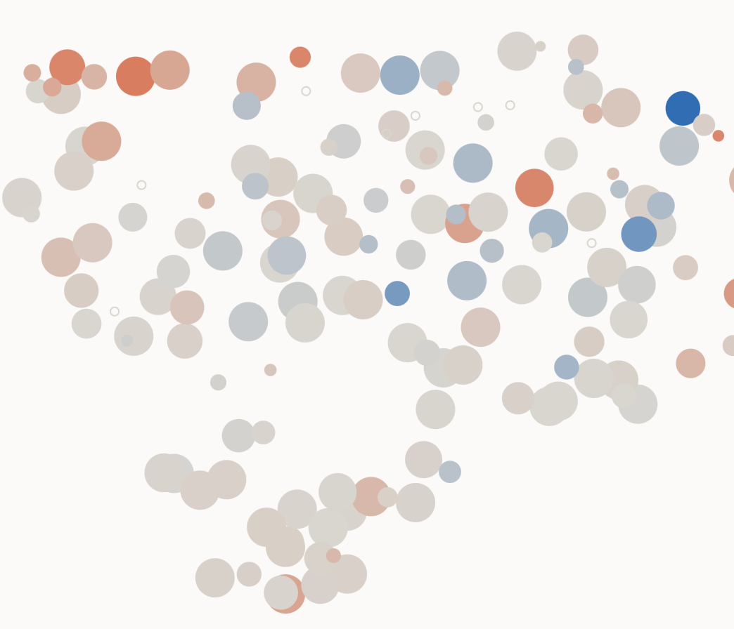
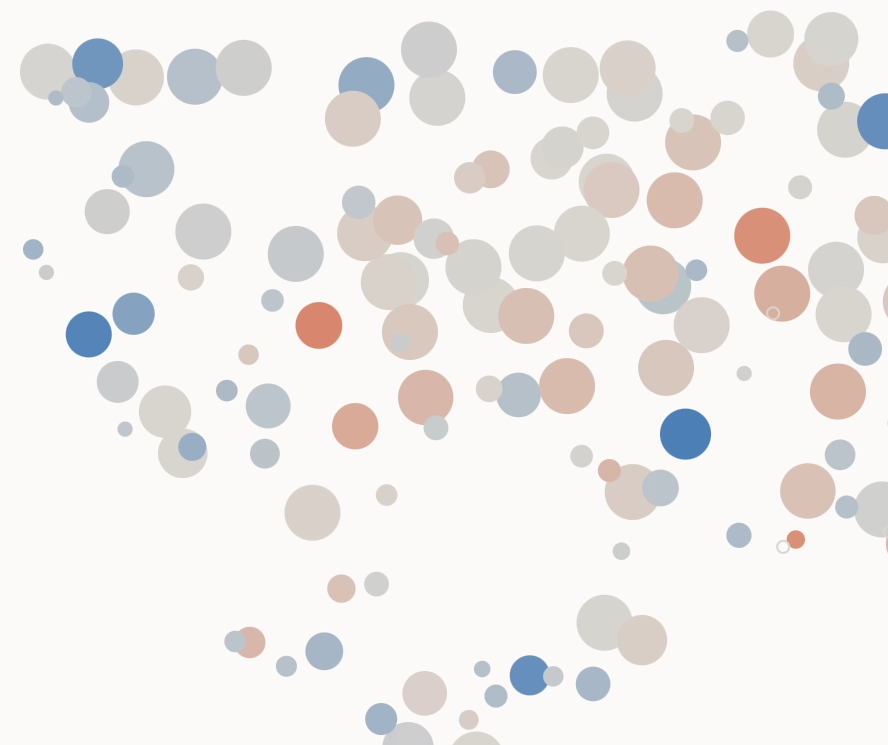
- Demand is not one number. Brands that share an audience share a preference: the same logo lifts sales for one group of brands and lowers them for another. The next model attributes those effects to the audience, not to chance.
Why a demand model
Simulation of consumer behaviour requires an understanding of demand. While it is tempting to say that the consumer is unpredictable, and that the same product marketed in different ways will face completely different demand, this is only partly true. Our experiments show that very basic features of a garment, such as colour, model (say, Chelsea boots) or logo, have a cumulative correlation of with the future sales of the product. In plain terms: these three features alone explain about a quarter of the variation in sales between garments, which is a lot for so little information.
While sales serve as the north star against which the parameters of the model are trained, the value is in the interpretation of the parameters, rather than in the sheer ability to predict revenue. Prediction in itself isn’t very valuable if one can’t extract actionable advice from the model. Therefore the emphasis of this article is on the way the results are interpreted. At the end of the article you can find a table with a breakdown of demand for common garment features in Europe in September 2026, such as colour, type, logo and pattern.
Data
The core part of demand modelling is sales data. As mentioned, we collect SKU-level sales data for European clothing brands. The raw sales we observe are , which form a 3D grid with a brand, product and time axis. Trend (time series) analysis is out of the scope of this investigation, therefore sales can be summed across the time dimension, leaving us with a sales table . Below you can see example rows from the sales dataset.
| Brand b | Product p | Sales in September sb,p |
|---|---|---|
| Adanola | Ultimate Pocket Leggings, Sea Green | 415 |
| Adanola | Modal Soft Rib Button Up Cardigan, Light Grey Melange | 35 |
| Mint Velvet | Black Satin Barrel Leg Trousers | 245 |
| Mint Velvet | Grey Ruched Detail High Neck Top | 4 |
While the sales of a product are the target variable the model is trained to predict, the predictors (the variables used as inputs to the model) are high-level features of the product. They include product family, type, colour, logo layout, pattern etc. Features were extracted by an LLM (Gemini Flash Lite) from the description of the product on the merchant’s website. For visual features such as pattern or logo layout, the product image was used. The complete set of product features is listed below.
| Feature | Levels | Reference level | Example values | Labelled from |
|---|---|---|---|---|
| Family | 10 | tops | bottoms, outerwear, footwear, one-piece, accessories, bags, jewellery | product text |
| Type (nested in family) | 105 | its family’s average | jeans, trousers, shorts · t-shirt, hoodie, shirt · sneakers, loafers, boots | product text |
| Colour | 21 | black | white, navy, beige, brown, olive, burgundy, multi | product text |
| Material | 17 | cotton | wool, linen, denim, leather, silk, cashmere, polyester | product text |
| Fit | 6 | regular | slim, relaxed, oversized | product text |
| Pattern | 7 | solid | stripe, check, print, graphic | product image |
| Logo | 4 | none | discreet, statement | product image |
| Gender | 5 | women | men, unisex, kids | product text |
Apart from the features of a product, we had a set of control variables. A control is a variable we put in the model not because we care about its own effect, but so it doesn’t distort the effects we do care about. Our controls include price, age (since first released), availability and the brand itself.
A careful reader can spot that advertising data is excluded from the modelling. The reasoning for this decision is that the reach of a specific ad (how many times the product was shown) is largely triggered by the well-selling features on modern advertising platforms such as Meta or Google, rather than by a deliberate brand decision. Thus, including ads may overshadow the true impact of a detail, wrongly attributing all the weight to the ad spend.
Model
In the modern consumer economy brands are heavily differentiated, which questions how comparable their product time series are. This is a common case of panel data. Panel data is characterised by partial separation, which leaves a data scientist wondering whether every subset of the data should be treated with a separate model (no pooling), or the data should be pooled together and a single model fitted on it (total pooling).
The right approach is partial pooling, powered by a random effects model (warning, technical details coming). There is room for variation between brands – some can only sell pink clothes – but brands do share a common trend – black is the most popular colour. Because sales are positive integers we model them as a Negative Binomial GLM with a log link function. (Poisson is too rigid with its variance = mean.)
For a single product by a brand , the sales in September are predicted as
or in log form:
- – the brand’s baseline: how much a typical product of this brand sells
- – the number of days the product was in stock
- – days since the product was published
- – the product’s features: 1 if it is, say, white or made of wool, otherwise 0
It can be seen that the parameters aren’t shared between brands directly, and for each feature , every brand has its own weight, . In fact, they aren’t completely separate, because the random effects model pulls them towards the average value across all brands by adding a penalty-for-deviation term to the log-likelihood:
Two important technical caveats, or rather technical choices, are:
- For the classes in category , only were explicitly used as dummies; one class was absorbed into the intercept for interpretability. For example, black was indicated through the absence of any other colour.
- Nested features (shoes → Chelsea) were avoided by collapsing the hierarchy and only using the final classes as inputs into the model.
Reading the parameters
After the model is fitted, the parameters have to be interpreted to provide an insight into the features leading to higher demand. From the model specification above, the following proportionality holds for any specific feature :
Thus, for a binary feature (either present or not) the impact on sales is represented by , where the parameter has been averaged across brands.
To take a concrete example, let’s consider the colour brown. Its coefficient in the model happens to be . Thus the effect compared against the base (black) is , meaning that brown sells 90% as much as black. Below you can see some of the findings the demand model was able to capture. The first column of numbers is the effect against the feature’s base level; the second is against the average product.
| Feature | Value | vs base level | vs average product | Reading |
|---|---|---|---|---|
| Colour · base: black | ||||
| black | 1.00 | 1.31× | Black sells 31% more than the average colour | |
| brown | 0.90 | 1.17× | ||
| navy | 0.88 | 1.15× | ||
| white | 0.72 | 0.94× | Close to average | |
| beige | 0.64 | 0.84× | ||
| pink | 0.55 | 0.72× | ||
| yellow | 0.41 | 0.53× | Yellow sells about half as much as the average colour | |
| Family · base: tops | ||||
| tops | 1.00 | 1.41× | ||
| bottoms | 0.98 | 1.37× | ||
| footwear | 0.80 | 1.13× | ||
| underwear & swim | 0.51 | 0.72× | ||
| accessories | 0.29 | 0.40× | Accessories sell 60% less than the average product | |
| Type · within family | ||||
| long-sleeve t-shirt | — | 2.78× | Strongest single type this month | |
| jeans | — | 2.46× | ||
| sneakers | — | 1.69× | ||
| dress | — | 0.75× | ||
| shorts | — | 0.64× | Seasonal: shorts in autumn | |
| Material · base: cotton | ||||
| wool | 1.19 | 1.15× | An autumn material sells better | |
| cotton | 1.00 | 0.97× | ||
| cashmere | 0.77 | 0.75× | Expensive, so fewer units | |
| linen | 0.44 | 0.43× | A summer material, out of season | |
| Pattern · base: solid | ||||
| solid | 1.00 | 1.07× | Plain products sell slightly better | |
| stripe | 0.85 | 0.91× | ||
| 0.81 | 0.87× | |||
| Logo · base: none | ||||
| none | 1.00 | 1.03× | ||
| statement | 0.84 | 0.86× | Big logos sell 14% less | |
| Fit · base: regular | ||||
| slim / relaxed / oversized | 0.99–1.02 | 1.01–1.04× | No effect: fit does not move sales | |
Next steps: demand per audience
So far, we have been talking about demand as a global property. We did allow for variation between brands, but it was explained by abstract brand differences rather than by the structural differences in the target audience of the brand. However, it is intuitive that there are audiences for which pink is trending, and audiences for which the trend for pink is negative. Thus an audience-aware model is needed, which attributes the “random” effects to the audience rather than to pure randomness.
A brand can be represented as a vector based on the composition of its target audience. Below you can see brands presented as two-dimensional vectors (projected down from higher abstract representations). If brands are close on the plot, they share a large chunk of their audience. On the diagram, the impact of logo presence or absence on demand is shown. It can be seen that the audiences of brands in one corner prefer an explicit logo, while the brands in the opposite corner observe exactly the opposite effect.
No logo
Explicit logo
Do you want to simulate your next product and marketing decisions? Talk to us.
developed at hugo
led by Arsenii Chistiakov