Absent sampling frame
At Hugo we work with reconstructing and simulating the consumer audiences. Inevitably this means we need to have accurate models of real world communities we are studying. However, no one in the world has an index of all the fans of specific clothing style, or even runners from an arbitrary city. While governments have relatively complete populations list, they absolutely lack the personal data to cluster those into meaningful communities. On the other end, consumer brands posses very scarce lists of their own customers which represent a tiny and highly skewed sample of their real target audience. In statistics, this is called absent sampling frame problem.
Chain Referral
However, the whole point and beauty of Datascience is that it is capable of finding workarounds in cases of missing or sparse data. Chain referral (or snowball sampling) is the common statistical method used to tackle the problem of the missing sampling frame. The idea is that, whilst we don’t know the whole population, but just a tiny fraction of it, we still can ask the known members to refer us to some more known members, and continue this recursion till we collect the target size of the dataset - say 10000 members.
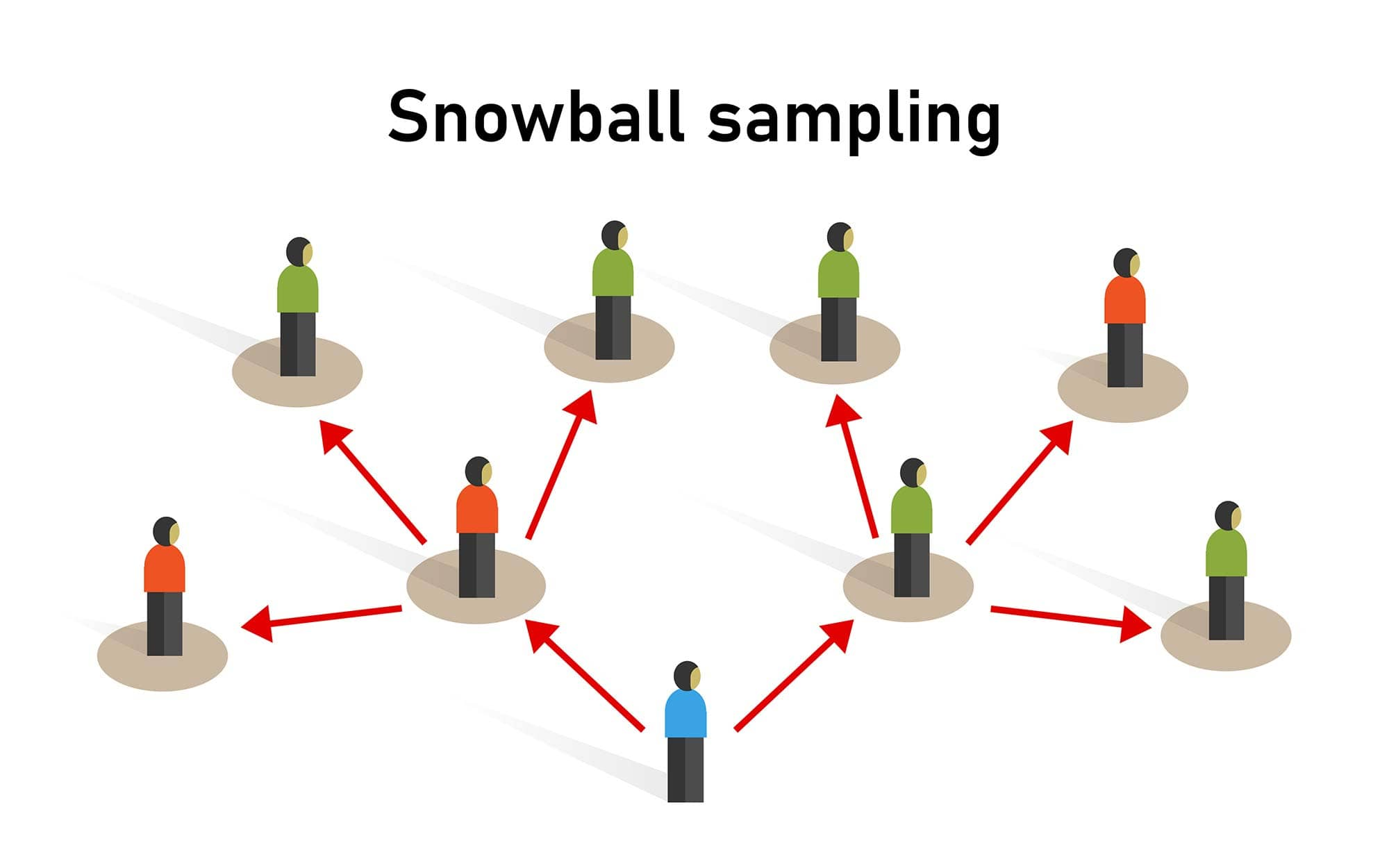
Historically it was considered unreliable, till the seminal paper by Heckathorn 2008, which looked into how exactly unreliable and biased the chain referral methods are, and how those flaws can be mathematically corrected for conclusions to be statistically sound. Specifically, the chain referral methods carry 2 strong bias which must be adressed:
- “Popular child” bias - the chain referral propagates through the person to person connections. Therefore, well connected people are more likely end up in your sample, because they simply have more pathways for our snowball to lead to them.
- Homophily bias - People are more likely to refer the same kind of people as them. If we want to understand the population of paris and in our seed of 10 people 5 are fashion models, we likely will end up with highly skewed picture of society where the fashion plays exaggerated role in parisian life.
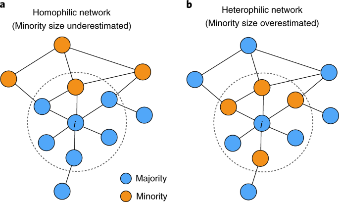
So how are those problems tackled by the statistics?
Addressing homophily bias
The homophily bias can be addressed by ensuring that the chain referral “walks” are long enough - meaning that we reach the depth of 4-5 referrals. If we start our study with a fashion model, she/he might refer us to 5 other fashion models, one of which works in a cafe and the other studies in university. Asking them for more Parisians will not only produce fashion people, but also cafe workers and fellow students in Sarbone. The 3rd iteration will be free of the fashion bias.
Addressing the “Popular child” bias
The depth of the chain referrals doesn’t fix the fact that well connected individuals stay overrepresented in our dataset. Therefore, whenever computing a statistic (any statistical judgement) upon our sample we must adjust it according to RDS-II Estimator formula.
- : The estimated proportion of the hidden population that possesses trait (e.g., the percentage of the population that is female).
- : is the “degree” or number of connections any specific individual has.
This way we can see if male are considerably more social then female and therefore are likely to be overrepresented in our sample. The estimator allows us to recover the true and unbiased gender split.
Application to Social Media
At Hugo, we don’t rely on the real human data, because of it’s scarceness and expansiveness. Instead we use social media platforms such as TikTok and Instagram to serve as representations of the real world and find the target communities in there.
Silent Respondents
Same absent sampling frame is present on social media, however the chain referral is complicated by the fact that we can’t “ask” an account to refer us to 10 more “inners”. Messaging accounts in automated manner violates the terms of service of platforms.
Therefore, we need an alternative way of getting the referrals to more and more members of community. One such way is followers and followings lists which are publicly available. We need to be able to iterate through that lists and verify each individual follower as an inner. One such way is to look at every account post and decided whether the account looks like he could be a member or not. For example, if we would be looking for runners in Brooklyn, we could check with LLMs if the user posts anything about running and living in Brooklyn.
2 Big Problems
Majority of members don’t post about them being a member in the community. Often times, filtering members by the explicit signal on social media leads to the most radical or agitated part of the group. Moreover, the majority of accounts can be, what we call “lurkers” - they might not post anything on social media and be consumers of the content of other influential members.
Moreover, the validation of posts require a costly LLM processing of images and videos. The videos are required for TikTok and instagram - highly visual platforms where basing judgements on texts leads to unpredictable bias - such as commercials. Average user doesn’t write anything informative. The cost is a problem because even a cost of 10 cents per validation of an account, would mean that collecting 10000 accounts (a representative sample of a medium size audience) would cost 1000€.
Therefore, the key for verification of members is to rely on topology of social graph - meaning who do you follow.
5 Parameters beat 1 Billion
I have spend a long time trying to understand what works as a good separator of members and outsiders of any arbitrary community. Some communities were very easy to detect, for example Ironmans. Ironmans follow Ironmans, shout in their descriptions that they are Ironmans, and don’t follow non-Ironmans. However, most of target audiences are much less clustered then Ironman community is. The common axis of the target audience include: country, gender, age, and hobby or a lifestyle.
The danger zone for classifying inners from outsiders are satelite audiences. If we care specifically about men in Germany, it’s quite easy to separate their following patterns from Italian ones, but it’s much harder to separate them from German women. They share in common a lot of news channels, organizations and influential figures. On the other hand, the name and profile picture can tell us a gender, which is a tie breaker in the specific case allowing to put the boundary between not only German men and the rest of the world, but also between them and German women.
Creating the Gold Sample
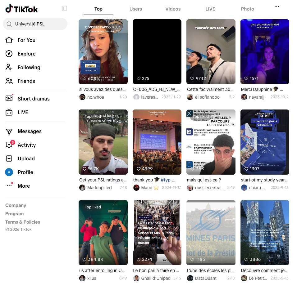
To understand who a “member” looks, we need to gather a set of validated members. We do this through searching TikTok or Instagram for keywords only locals would mentions such as “Étudier à l’Université PSL”. We make sure to pick the seed queries without of strong bias towards any specific population. This way, we collect a sample of 100-200 inners, using light weight large language models to verify the membership of the seeds. The sample size might seem surprisingly small, but it is explained by the fact that the modeling task isn’t abstract, and is rather simple in the geometrical sense.
Importantly, we collect samples for a list of anti-targets. In case of Ironman those anti-targets good be gym athletes or simply runners. We must learn features which separate those closely relate but separate audiences. Additionally we use a random sample from our database of all audiences we collected before to represent background.
We turn those accounts into datapoints, by deriving a list of features for each individual account. Those features can be grouped into to approximate categories: graph features and profile features.
Graph Features
After obtaining the Gold Sample, we expand those accounts by checking who do they follow. This creates a social graph object which represent all the interconnections within the sample and outside of it (to some influential figures). We also create anti-maps - social graphs of the anti-target audiences.
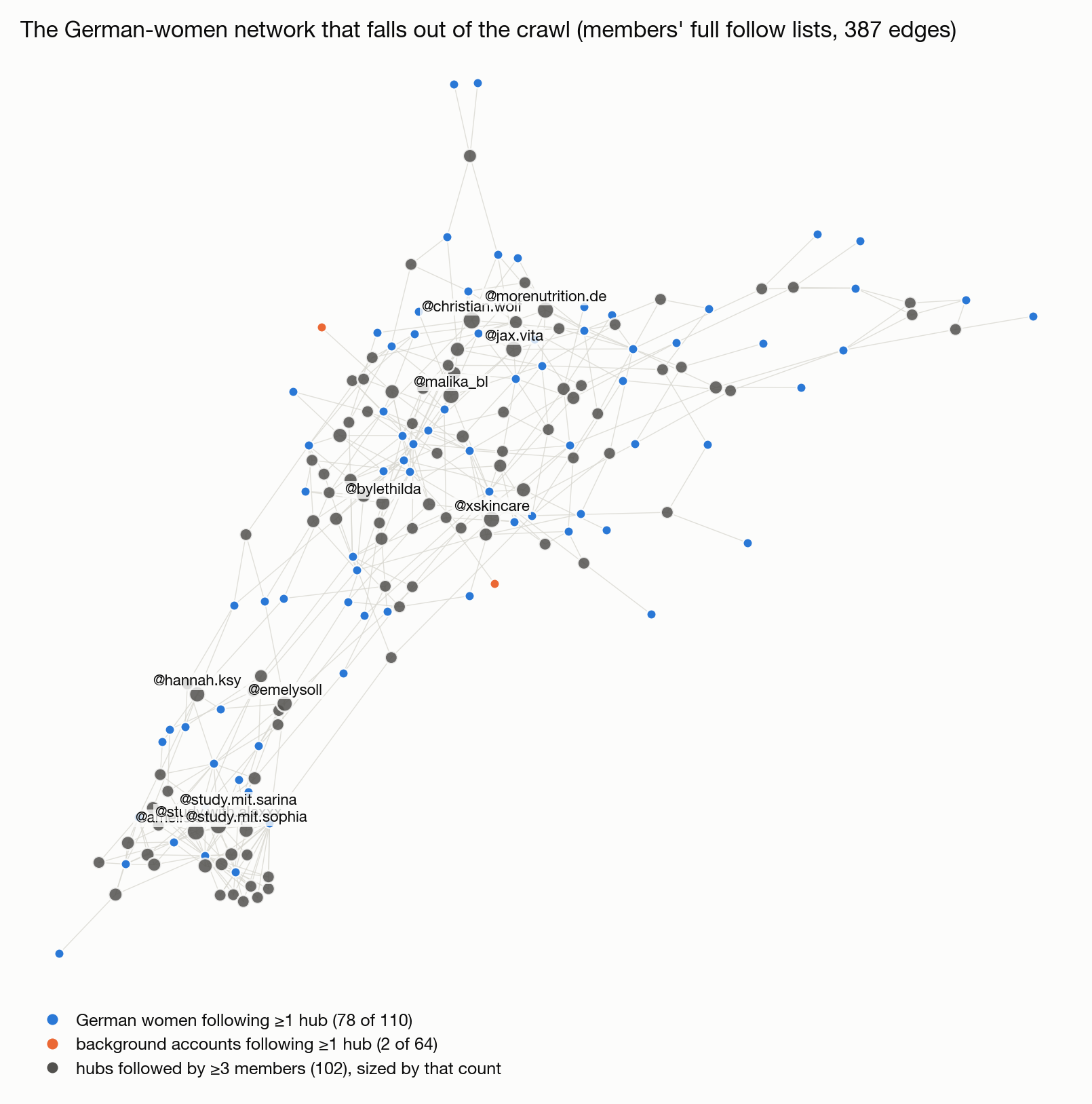
Now a newcomer - an account obtained from the follower or following list of some of the members - gets their followings checked and projected onto this gold sample graph. We compute degree centrality - a fancy term for the number of raw overlaps of accounts present in the graph and accounts follower by the newcomer. This simple metric does 90% of the job separating the members and outsiders. The members score 10 times higher on it.
Moreover we compute the degree centrality on the negative maps - meaning how many accounts from the anti-targets map the account is following. This is specifically designed to identify the satelite audiences and filter them out.
Apart from degree centrality we compute other complex graph metrics, such as PageRank and Eigenvector centrality which can be helpful in some edge cases but usually don’t bring much new to the table not captured by the degree centrality.
Profile Features
However, for some anti-targets the purely topological features might not be enough. because of heavy overlap of male and female following maps (male tend to follow female, more then male 😏) additional features are needed. Gender and Ethnicity estimation from name and profile picture were chosen, because of their availability. They help to separate male and female audiences, runners in a specific country from runners globally, completing the loop of the model.
Linear model
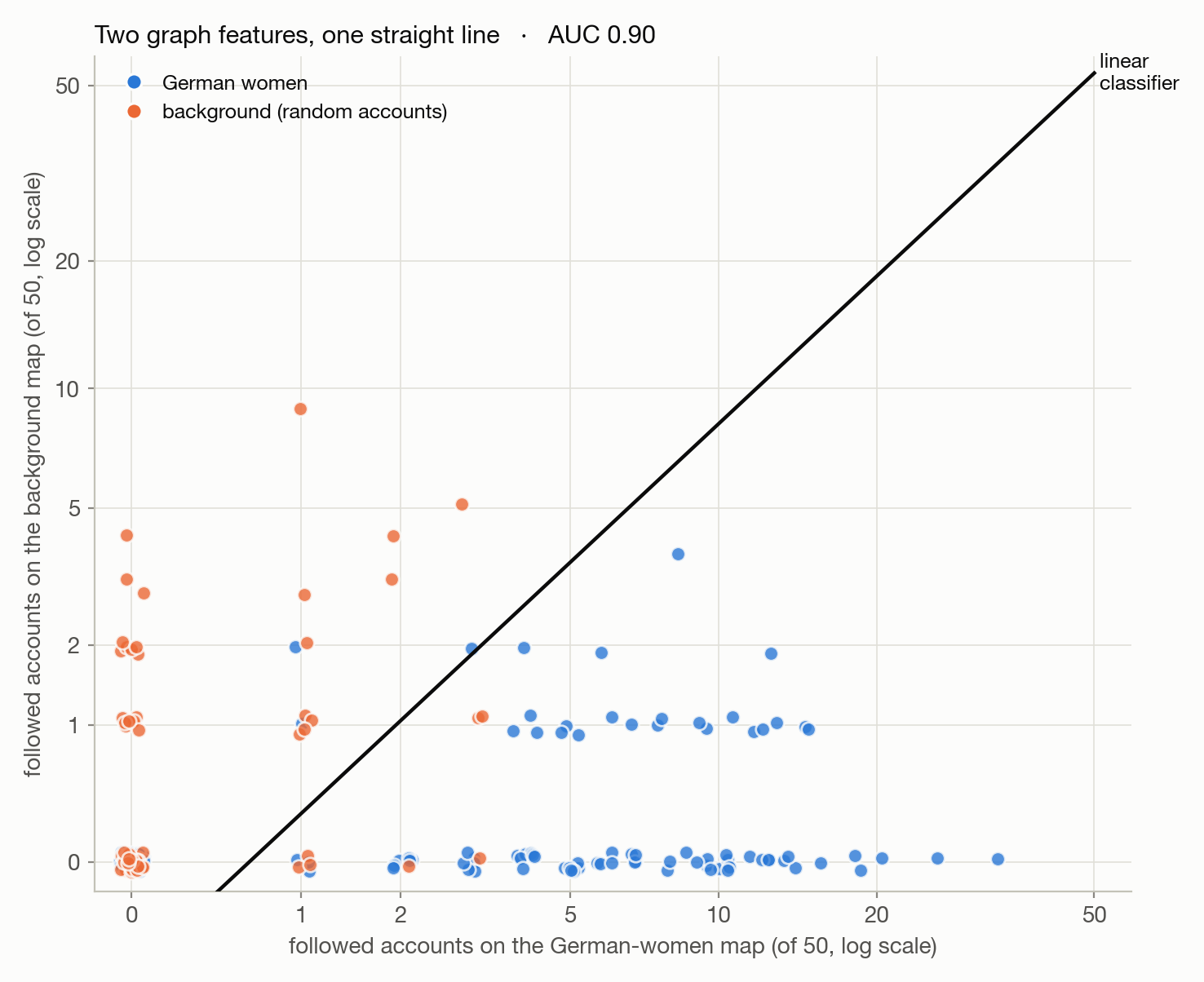
On top of the above explained features we run a linear classifier model. This simple model is capable of detecting lurkers at the price and information amount much lower then the LLM is, allowing us to power the social media chain referral and collect the large samples of arbitrary target audience at a very low price.
The visualization on the left shows just 2 features and how they allow to separate German Women audience from the background.