How we are able to map out any audience

Absent sampling frame

At Hugo we reconstruct and simulate consumer audiences. Inevitably that means we need accurate models of the real communities we are studying. No one in the world holds an index of every fan of a specific clothing style, or even of the runners in a given city. Governments hold relatively complete population lists, but they lack the personal data needed to cluster those people into meaningful communities. Consumer brands, at the other end, hold very thin lists of their own customers, which represent a tiny and heavily skewed sample of their real target audience. In statistics this is called the absent sampling frame problem.

Chain referral

The point of data science is that it finds workarounds when data is missing or sparse. Chain referral, also called snowball sampling, is the common statistical method for the absent sampling frame. The idea is that even though we do not know the whole population, only a tiny fraction of it, we can still ask the members we do know to refer us to more members, and repeat that recursion until we reach the target size of the dataset, say 10,000 members.

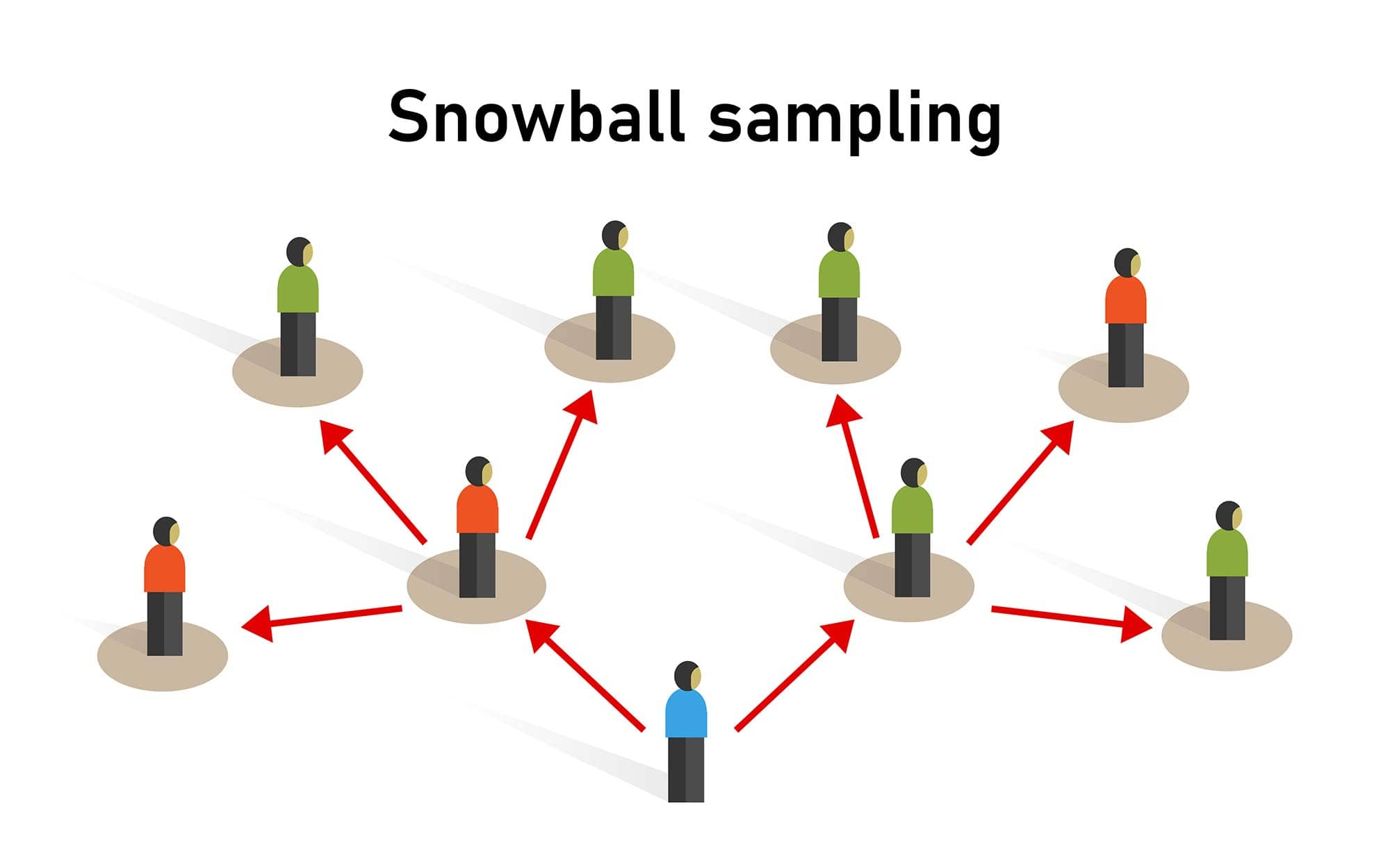
Historically the method was considered unreliable, until Douglas Heckathorn set out exactly how biased chain referral is and how the bias can be corrected for, so that conclusions drawn from a referral chain are statistically sound. Respondent-Driven Sampling II (Social Problems, 2002) is where the correction and the RDS-II name come from; Probability Based Estimation Theory for Respondent Driven Sampling (Volz and Heckathorn, Journal of Official Statistics, 2008) derives the estimator below as an ordinary survey-sampling estimator rather than a special case. Chain referral carries two strong biases, and both have to be addressed.

• “Popular child” bias. Chain referral propagates through person-to-person connections, so well-connected people are more likely to end up in the sample: they simply offer more pathways for the snowball to reach them.
• Homophily bias. People are more likely to refer people like themselves. If we want to understand the population of Paris and five of the ten people in our seed are fashion models, we will end up with a heavily skewed picture of a city in which fashion plays an exaggerated role.

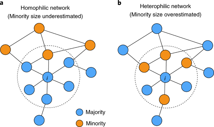
So how does statistics tackle those two problems?

Addressing homophily bias

Homophily bias can be addressed by making sure the chain referral “walks” run long enough, meaning that we reach a depth of four or five referrals. If we start our study with a fashion model, they might refer us to five other fashion models, one of whom works in a cafe and another of whom studies at university. Asking those two for more Parisians produces not only fashion people but also cafe workers and fellow students at the Sorbonne. By the third iteration the fashion bias is gone.

Addressing the “popular child” bias

Walking deeper does not fix the fact that well-connected individuals stay overrepresented in the dataset. So whenever we compute a statistic on the sample, any statistical judgement at all, we have to adjust it with the RDS-II estimator.

• ${\hat{P}}_A$: the estimated proportion of the hidden population that has trait $A$, for example the share of the population that is female.
• $d_i$: the degree, or number of connections, of a specific individual.

This way we can see whether men are considerably more social than women and therefore likely to be overrepresented in our sample. The estimator lets us recover the true, unbiased gender split.

Application to social media

For the reasons above, we do not collect data from people directly. Instead we use social media platforms such as TikTok and Instagram as representations of the real world, and find the target communities there.

No one to ask

The same absent sampling frame problem exists on social media, but chain referral is complicated by the fact that we cannot “ask” an account to refer us to ten more members. Messaging accounts in an automated way violates the platforms’ terms of service.

So we need another way to get referrals to more and more members of a community. One is the follower and following lists, which are publicly available. We need to iterate through those lists and verify each follower as a member. One way to do that is to look at every post on an account and decide whether the account could belong to a member. For example, if we were looking for runners in Brooklyn, we could use an LLM to check whether the user posts anything about running or about living in Brooklyn.

Neither bias from the survey case goes away on a follow graph. Homophily is still handled by depth: a crawl that stops at the first wave returns the seeds’ own neighbourhoods and inherits whatever the seed queries leaned towards, so the walk has to run the same four or five waves out. The degree bias gets easier rather than harder. Degree is the one quantity a platform states outright, so instead of asking an account how many people it knows we read its following count, and the RDS-II weighting can be applied to the finished sample directly.

Two big problems

Reading posts to decide membership fails on two counts.

The first is silence. Most members never post about being part of the community, so filtering on explicit signal surfaces only the most radical or most vocal part of the group. Most accounts are what we call lurkers: they post nothing themselves and only consume the content of more influential members. Those are the silent respondents, and a method that reads posts cannot see them at all.

The second is cost. Validating posts requires LLM processing of images and video. Video is unavoidable on TikTok and Instagram, highly visual platforms where judging an account on its text alone introduces unpredictable bias, commercial posts being one example. The average user writes nothing informative. At ten cents per account validated, collecting 10,000 accounts, a representative sample of a medium-sized audience, would cost €1,000.

So the key to verifying members is to rely on the topology of the social graph, meaning who an account follows.

Five parameters beat a billion

We spent a long time working out what separates the members of an arbitrary community from the outsiders. Some communities are very easy to detect, Ironman athletes for example. Ironman athletes follow other Ironman athletes, announce it in their bios, and follow almost no one outside the sport. Most target audiences are far less clustered than the Ironman community. The common axes of a target audience are country, gender, age, and a hobby or a lifestyle.

The danger zone when separating members from outsiders is satellite audiences. If we care specifically about men in Germany, it is quite easy to separate their following patterns from Italian ones, but much harder to separate them from those of German women. The two groups share a lot of news channels, organizations and influential figures. A name and a profile picture, though, tell us a gender, and in that specific case gender is the tie breaker: it draws a boundary not only between German men and the rest of the world, but also between German men and German women.

Creating the gold sample

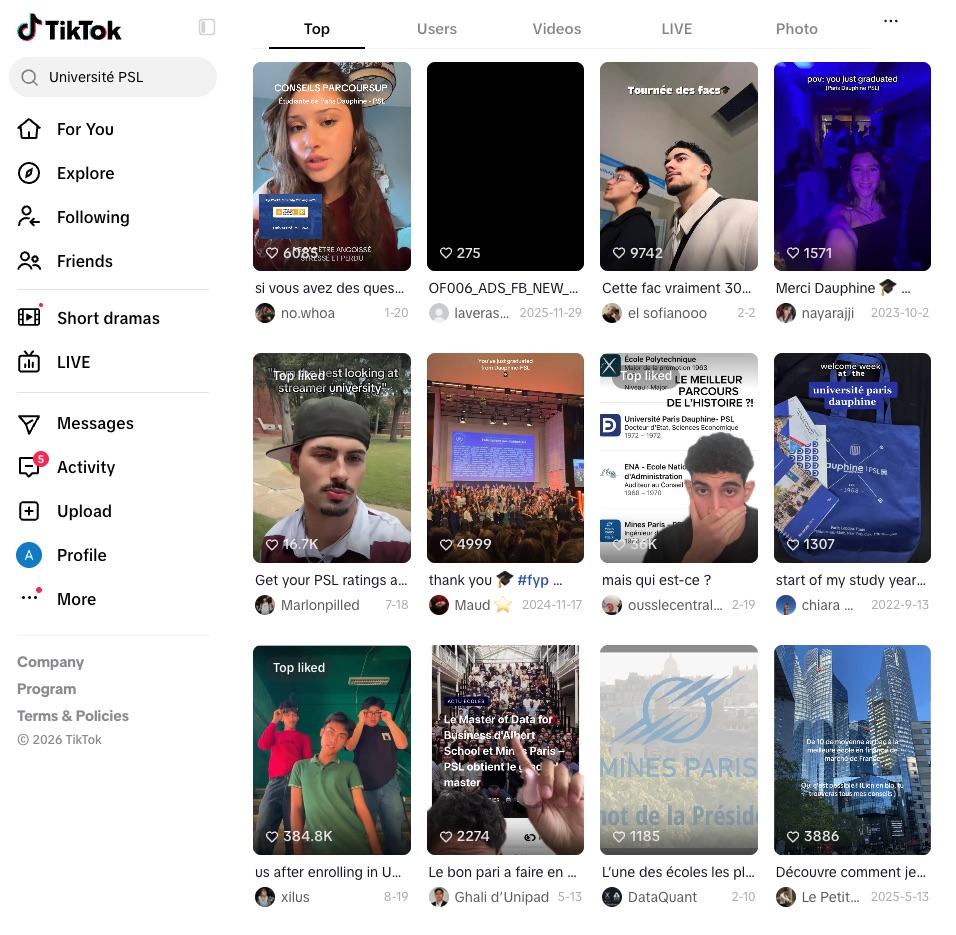
To understand what a “member” looks like, we first gather a set of validated members. We do this by searching TikTok or Instagram for phrases only locals would use, such as “Étudier à l’Université PSL”. We pick seed queries with no strong bias towards any specific part of the population. That gives us a sample of 100 to 200 members, with lightweight language models verifying the membership of each seed. The sample size may look surprisingly small, but the modeling task is not abstract: it is simple in the geometrical sense. Members and outsiders end up in different places, and a straight line is enough to tell them apart, which is what the plot at the end of this piece shows.

We also collect samples for a list of anti-targets. In the case of Ironman, those anti-targets could be gym athletes or ordinary runners. We need features that separate those closely related but distinct audiences. And we take a random sample from our database of every audience we have collected before to represent the background.

We turn those accounts into datapoints by deriving a list of features for each individual account. The features fall into two rough categories: graph features and profile features.

Graph features

After obtaining the gold sample, we expand those accounts by checking who they follow. This creates a social graph object that represents all the interconnections inside the sample and outside it, out to some influential figures. We also build anti-maps: social graphs of the anti-target audiences.

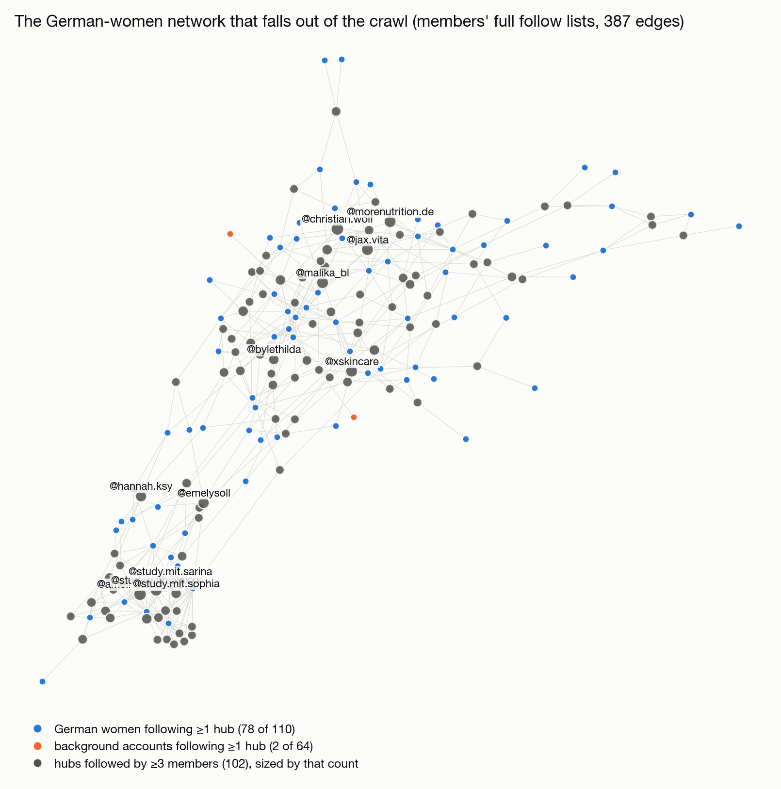
A newcomer, an account taken from the follower or following list of one of the members, then has its own followings checked and projected onto this gold sample graph. We compute degree centrality, a fancy term for the raw number of overlaps between the accounts in the graph and the accounts the newcomer follows. This simple metric does 90% of the job of separating members from outsiders. Members score ten times higher on it.

We compute degree centrality on the negative maps too, meaning how many accounts from the anti-target maps the newcomer follows. That is designed specifically to identify satellite audiences and filter them out.

Alongside degree centrality we compute other, more complex graph metrics, such as PageRank and eigenvector centrality. Those help in some edge cases, but they usually add little that degree centrality has not already captured.

Profile features

For some anti-targets, though, purely topological features are not enough. Because male and female following maps overlap heavily (men tend to follow women more than they follow men 😏), additional features are needed. We estimate gender and ethnicity from the name and the profile picture, chosen because they are almost always available. They help separate male from female audiences, and runners in a specific country from runners globally, which closes the loop of the model.

Linear model

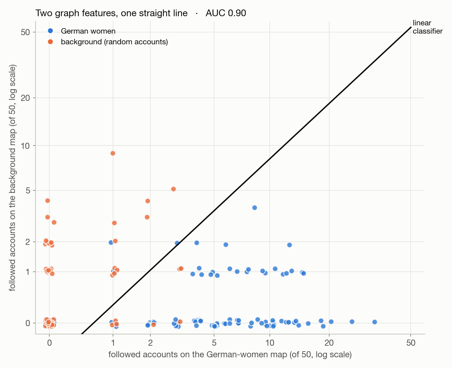
On top of the features above we run a linear classifier. Five features go into it:

• overlap with the gold sample graph
• overlap with the anti-target maps
• overlap with the background map
• gender, estimated from name and profile picture
• ethnicity, estimated from name and profile picture

The visualization on the left shows two of those five, and how far they get on their own: German women to the right, background accounts near zero, one straight line between them at AUC 0.90.

That is the whole model. It detects lurkers at a far lower price, and on far less information, than an LLM needs, which is what lets us run chain referral on social media and collect large samples of an arbitrary target audience cheaply.

Put together, that is how we get from a keyword search to a fully mapped community. The seed query is the only part that changes between audiences: the follow-graph crawl, the anti-maps and the classifier run the same way for runners in Brooklyn as they do for German women. What comes out is a representative sample of 10,000 real people’s accounts, reached through real connections, including the ones who never post anything themselves, for a fraction of the cost and the time it would take a research agency.

That is what lets us analyze and simulate an audience.