Our First Revenue Simulation Model

No existing model is trained on revenue, so we are training our own. The first one removes 40% of the uncertainty in launch revenue compared to predicting historic averages.

At Hugo, our mission is to perfectly predict and simulate consumers. One of the most valuable problems to solve for is to simulate how much revenue a company will make from any product, marketing, or branding decision – before they act. We call this Revenue Simulations. No existing model is trained on revenue – which is the reason we are training our own Revenue Models to use in our simulations. This article covers our first revenue model which eliminates 40% of the uncertainty in revenue compared to predicting historic averages.

How the model can be applied to your business

Before going into how we trained the model, we thought it was appropriate to start with a use-case. The model can be applied to simulate the revenue of a new product launch before it happens. If you are a fashion brand for example, we can apply our revenue simulation to estimate the demand, revenue, and units sold on every new piece of clothing or shoes before it is released to consumers – it will not be a perfect estimation, but far better than any other alternative. This helps you:

Know which products to prioritize your marketing efforts on.
Estimate how much inventory you need to keep of every new product.
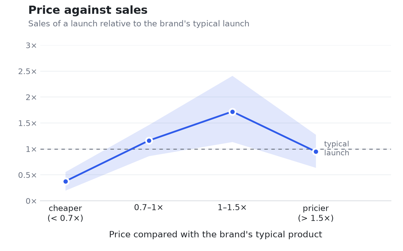
Test how different prices change the forecast.

Revenue is our loss function

Training large statistical models requires a loss function – an objective which the model learns. Sales and revenue are the target consumer brands optimize for. Hence, sales data of products will serve as such an objective for Hugo’s consumer simulations. One could consider brand image being a contradiction to that rule; however, it is nothing else but a predictor of the revenue of a brand in the long run. Sales serve as a grounding for the simulation, allowing the learned behavior to be not only “believable”, but also realistic.

This requires us to constantly acquire more sales data to train our models on. Additionally, when working with a brand we can take their internal historical data into account for the model we apply for them.

Why not questionnaires

While opinions and questionnaires are currently used by both classical consumer research and simulation labs as the main tool for understanding customer groups, this focus on artificial features contradicts “The Bitter Lesson”.

An analogy that might be helpful here is the classification of images, for example the task of classifying cats and dogs. This is a classic example of human handcrafted heuristics being surpassed by Deep Learning. The key idea of Deep Learning is simple: remove all handcrafted features – such as questionnaires and opinion spreadsheets – and allow the model to come up with its own abstract features, which help it tell cats from dogs.

But questionnaires violate yet another rule of “The Bitter Lesson”. They don’t scale. In 2026, the number of publicly available questionnaires (which accounts for the majority of existing ones, and costs enormous money to create) is about 3,000. Those numbers are incompatible with Deep Learning. Even more so, questionnaires don’t generalize. Asking a person why they bought specific jeans, you should expect an honest response: “They look fly”.

The Bitter Lesson of Statistics

Outsmarting yourself

When working in social data science, there is a bitter lesson of its own – call it “The Bitter Lesson of Statistics”. Usually, the linear model performs better than the smart one: Linear Regression, Linear Classification, Generalized Linear Model. One feels quite foolish when realizing that a Graph Neural Network trained through Reinforcement Learning is outperformed by a linear regression on 3 parameters.

Thus we start simple

Following “The Bitter Lesson of Statistics”, we decided to start simple. How do you predict the revenue in the following time period of a new product launch? Well, the simplest thing one could do is to look at the revenue of a previous product drop and predict the same. Turns out this already gets you surprisingly far, and serves as an amazing benchmark for whatever successor model we would use. Building on that same idea, with a few well-chosen drivers added, our first model removes 40% of the uncertainty compared to predicting historic averages.

R² is the success metric

If the mean serves as a base, then R² serves as the metric for a future model to understand the improvement in simulating revenue. This score tells how much uncertainty the model has removed in predicting the revenue of a launch when compared to predicting the historic average. So far, we have been using Poisson regression (a generalized linear model) on a set of internal brand sales data, marketing, pricing, and product features data, which has gotten us to an R² of 0.4 across 207 launches of 20 brands.

Beautiful Linear Model

When pondering one’s purchasing behavior, it becomes obvious that the final decision to buy something is a combination of infinitely many factors. When modeling mass behavior across a target audience, these manifest as complex, abstract consumer patterns. While perfectly capturing every nuance requires mapping all latent behavioral shapes, a few primary factors are significant enough to give us a remarkably accurate picture of sales.

For example, exposure drives conversion: the more a potential customer encounters a product, the more likely they are to buy. Adding a term to represent even a single major lever like exposure yields a massive improvement over simply predicting historical averages.

To build our baseline sales simulation model, alongside exposure, we incorporated predictors for launch scale, perceived product and brand value, and preceding sales volume – guided by the expectation that future success correlates with current momentum. Crucially, we pair these drivers with a dynamic time-step trajectory to capture how sales volume naturally decays post-release.

Figure 1: Launches priced 1–1.5× above the brand’s typical product sell about 1.7× a typical launch. Much cheaper launches sell less than half. The shaded band shows the uncertainty.

Preventing Overfitting with Ridge Regularization

Because these features can overlap, we apply Ridge regularization (L2 penalty) during model fitting. This prevents any single driver from dominating the predictions and keeps our coefficients stable across different brands.

Testing True Generalization

To ensure our simulation isn’t simply memorizing past drops, we rigorously evaluate it using Leave-One-Brand-Out validation – training the model on all other brands and forecasting an entirely unseen brand’s launch performance from scratch.

The Power of a Simple Baseline

Despite its simplicity, this baseline successfully eliminates 40% of the uncertainty in launch revenue compared to predicting historic launch averages.

The dominant drivers act as major anchors. We expect that when a far more complex model is trained on huge amounts of data, it will naturally learn and internalize these underlying dynamics on its own. In the meantime, however, we can achieve surprisingly strong predictive power simply by fitting a couple of well-chosen parameters to model these major ideas directly. Most importantly, it gives us a rigorous benchmark to evaluate whether a complex model has truly succeeded in internalizing the underlying dynamics.

Want to simulate your next product’s revenue before it is released? Talk to us.

developed at hugo

led by Ilari Sell

Appendix: Formal Model Architecture & Mathematics

This section provides the mathematical formulation for readers interested in the underlying statistical mechanics of our baseline model.

1. Model specification

We model unit sales $y_{i, t}$ at discrete time step $t \in T_{i}$ post-release for launch $i$ using a Ridge-penalized Poisson Generalized Linear Model (GLM) with a log-link function:

y_{i, t} \sim Poisson (μ_{i, t})

\ln μ_{i, t} = \ln L_{i} + γ_{t} + \sum_{k = 1}^{K} β_{k} \cdot z (X_{k, i})

In vector notation:

\ln μ_{i, t} = \ln L_{i} + γ_{t} + 𝜷^{⊤} z (𝐱_{i})

Notation reference:

$y_{i, t}$ : Observed unit sales for launch $i$ during time step $t$ .
$L_{i} > 0$ : Baseline demand offset for launch $i$ , capturing brand-level velocity (coefficient fixed at 1).
$γ_{t}$ : Time-step fixed effect relative to the reference launch step $t = 0$ .
$𝐱_{i} = [X_{1, i}, \dots, X_{K, i}]^{⊤}$ : $K$ -dimensional vector of launch covariates.
$z (X_{k, i})$ : Standardized feature value computed on the training fold.
$𝜷$ : Regression coefficients corresponding to the $K$ standardized features.

2. Loss function & parameter estimation

Parameters are estimated via maximum regularized log-likelihood with an L2 (Ridge) penalty applied to the feature coefficients $𝜷$ to handle multicollinearity:

(\hat{γ}, \hat{𝜷}) = \arg \max_{γ, 𝜷} \sum_{i = 1}^{N} \sum_{t \in T_{i}} [y_{i, t} \ln μ_{i, t} - μ_{i, t}] - λ ‖ 𝜷 ‖_{2}^{2}

where $‖ 𝜷 ‖_{2}^{2} = \sum_{k = 1}^{K} β_{k}^{2}$ , and $λ \geq 0$ is the regularization hyperparameter controlling coefficient shrinkage. The brand baseline $L_{i}$ and time-step effects $γ$ remain unpenalized.

3. Out-of-sample forecasting & metrics

The forecasted total launch volume ${\hat{y}}_{i}$ over the evaluation timeframe $T_{i}$ is the sum of step-level expectations:

{\hat{y}}_{i} = \sum_{t \in T_{i}} {\hat{μ}}_{i, t}, where {\hat{μ}}_{i, t} = L_{i} \exp ({\hat{γ}}_{t} + {\hat{𝜷}}^{⊤} z (𝐱_{i}))

Model accuracy is evaluated out-of-sample using Leave-One-Brand-Out (LOBO) cross-validation, calculated via $R^{2}$ against the baseline launch mean $\overline{y}$ :

R^{2} = 1 - \frac{\sum_{i = 1}^{N} (y_{i} - {\hat{y}}_{i})^{2}}{\sum_{i = 1}^{N} (y_{i} - \overline{y})^{2}}

Our first revenue simulation model